Table of Contents
- The curve
- Explore the curve and the book
- Compare the Moroccan sovereign curve
- The book
- The calculations
- The duration hedge
- The duration-plus-convexity hedge
- The key-rate hedge
- Size, liquidity and financing
- Out-of-sample: does the hedge survive a moving curve?
- Move the curve yourself
- Limitations
- Reproducibility
In one paragraph. On 16 October 2026, Bank Al-Maghrib’s reference curve ran from 2.13% at the three-month bill to 4.38% at the 28.5-year bond. I fitted a Nelson-Siegel-Svensson curve (3.85 bp in-sample; 30.6 bp leave-one-out, so the fit is thin and I say so), priced eight sovereign lines off it (81.4M MAD market value, 6.99 modified duration, 58.4k MAD per basis point of DV01, 8.21B of dollar convexity), and hedged the book four ways. Duration-only zeroes total DV01 with a 76.9M MAD short in the 8.7-year line — but turns a broadly spread key-rate profile into a -42.9k MAD/bp exposure at that single point and leaves 3.40B of convexity. Duration-plus-convexity zeroes both with a 5Y/18.8Y pair; a +100 bp belly move at 12.76Y still produces +369k MAD. A six-line key-rate hedge (3.5Y to 28.5Y) cuts the belly P&L to +86k, is 95% executable under a 10M-per-line cap versus 13% for the duration short, and in a 106-day out-of-sample backtest cuts daily P&L volatility from 112k to 6k MAD. The duration-only hedge leaves 50k and still has the largest residual among the hedges. The hedge changes the risk. It does not delete it. Every number above is derived from the formulas and worked arithmetic in The calculations.
Résumé (français). Le 16 octobre 2026, la courbe de référence de Bank Al-Maghrib allait de 2,13 % à 3 mois à 4,38 % à 28,5 ans. J’ai ajusté une courbe Nelson-Siegel-Svensson (RMSE 3,85 pb in-sample, 30,6 pb en validation croisée), pricé huit lignes souveraines (81,4 M MAD, duration modifiée 6,99, DV01 58,4k MAD/pb, convexité en dirhams 8,21 Md), puis construit quatre couvertures. Une seule jambe de duration annule le DV01 total mais concentre le risque sur le point 8,7 ans et laisse 3,40 Md de convexité. Une couverture duration + convexité annule les deux mais laisse +369k MAD sur un choc de ventre à 12,76 ans. Une couverture key-rate à six lignes (3,5 à 28,5 ans) ramène ce choc à +86k, est exécutable à 95 % sous un plafond de 10 M par ligne (contre 13 % pour la jambe unique), et réduit la volatilité quotidienne du backtest de 112k à 6k MAD. Le code, les données et le simulateur interactif sont reproductibles à partir de la même source.
The curve
Morocco’s sovereign curve is where the country’s rate risk is actually priced, and Bank Al-Maghrib publishes a clean daily reference: the Taux de référence des bons du Trésor on the secondary market, with a CSV export per value date.
The 16 October 2026 curve is upward sloping and steep at the front end: 10 observed points from 0.08 to 28.53 years, 2.13% to 4.38%. I fitted a Nelson-Siegel-Svensson curve by grid-searching the two decay constants and solving for the four factor loadings linearly at each pair:
| Maturity | Years | BAM yield | NSS fit | Residual |
|---|---|---|---|---|
| 16 Nov 2026 | 0.08 | 2.130% | 2.139% | +0.95 bp |
| 15 Feb 2027 | 0.33 | 2.200% | 2.176% | -2.37 bp |
| 16 Aug 2027 | 0.83 | 2.290% | 2.315% | +2.55 bp |
| 14 Feb 2028 | 1.33 | 2.470% | 2.461% | -0.90 bp |
| 15 Apr 2030 | 3.50 | 2.890% | 2.879% | -1.08 bp |
| 20 Oct 2031 | 5.01 | 3.090% | 3.091% | +0.08 bp |
| 18 Jun 2035 | 8.68 | 3.480% | 3.528% | +4.82 bp |
| 18 Jul 2039 | 12.76 | 3.950% | 3.865% | -8.50 bp |
| 14 Aug 2045 | 18.84 | 4.090% | 4.150% | +5.96 bp |
| 19 Apr 2055 | 28.53 | 4.380% | 4.365% | -1.51 bp |
The in-sample RMSE is 3.85 bp, with the largest miss at 12.76 years. That number is less impressive than it looks. Six parameters on ten points leave four residual degrees of freedom; the condition number of the normal equations is about 1.1 × 10⁷; the residual standard error is 6.1 bp; and the parameter standard errors are large (b₂ 1.03%, b₃ 0.79%, τ₁ 0.35, τ₂ 0.52). The honest test is leave-one-out: the NSS LOOCV RMSE is 30.6 bp, driven by the 28.5-year point (85.5 bp) and the three-month bill (26.3 bp). A four-parameter Nelson-Siegel curve has a slightly worse in-sample fit (4.23 bp) but a much better LOOCV (8.87 bp).
| Model | Params | In-sample RMSE | Max miss | LOOCV RMSE |
|---|---|---|---|---|
| NSS | 6 | 3.85 bp | 8.50 bp | 30.58 bp |
| Nelson-Siegel | 4 | 4.23 bp | 9.24 bp | 8.87 bp |
I keep the NSS curve for continuity, but I do not treat it as a forecasting model. Every hedge below is re-solved under the four-parameter NS curve: the duration short moves from 76.94M to 77.03M, residual convexity from 3.39B to 3.40B, the six-line key-rate residual DV01 stays at zero, and the +100 bp belly P&L moves from +86.0k to +86.0k. The conclusions are not a product of the NSS overfit.
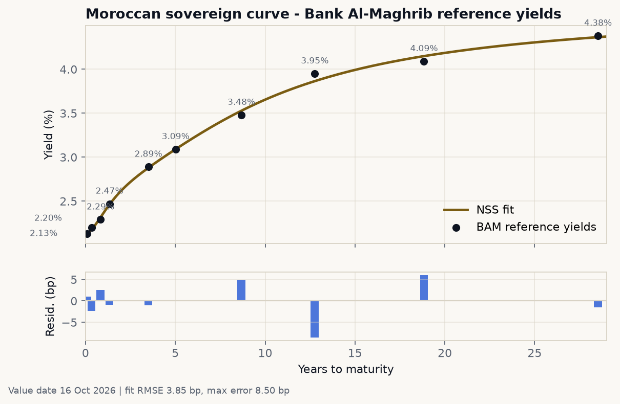
The fitted curve is smooth through the front end and undershoots the 12.76Y reference point by 8.5 bp. All pricing downstream uses the fitted curve, not the observed points.
Explore the curve and the book
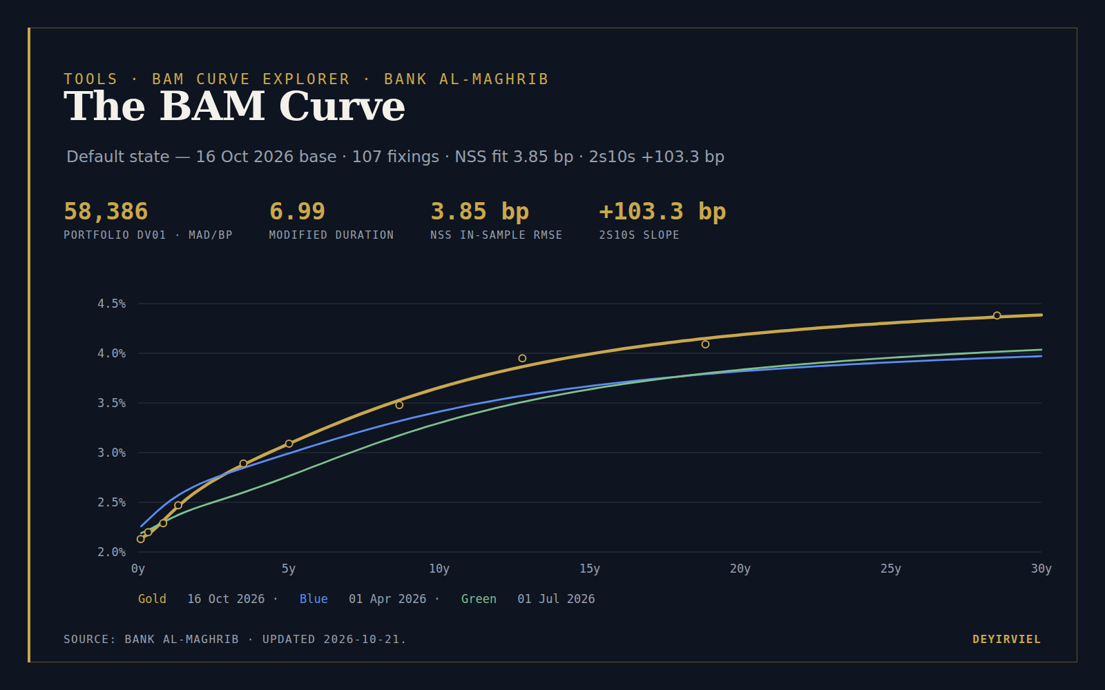
The explorer uses the same Bank Al-Maghrib CSV, the same NSS fit and the same bond analytics as the Python engine. It defaults to the published 16 October 2026 curve and compares it with 1 April and 1 July 2026. The date selector exposes every cached fixing; the bond estimator shows the dirty price, YTM, Macaulay and modified duration, convexity and curve DV01 for the chosen reference line. Historical dates hold the reference decay constants fixed, the same convention as the backtest.
BAM Curve Explorer · Bank Al-Maghrib
Compare the Moroccan sovereign curve
Curve metrics
- NSS fit RMSE
- —
- 2s10s
- —
- 3m10y
- —
- 5s30s
- —
- 2s30s
- —
- Curvature
- —
Bond estimator
- Dirty price
- —
- YTM
- —
- Macaulay
- —
- Modified duration
- —
- Convexity
- —
- Curve DV01
- —
Selected curves
| Date | 2s10s | Δ 2s10s | 3m10y | 5s30s | 2s30s | Curvature |
|---|
Chart loads when visible
Chart loads when visible
Charts unavailable. The tables above remain valid.
Methodology
Data and refresh
The source is Bank Al-Maghrib’s Taux de reference des bons du Tresor CSV export for the secondary market. The scheduled refresh downloads new weekday fixings intoscripts/tools/data/bam/, validates the value date and observation count, and keeps every existing file. If the BAM page or CSV export is unavailable, the builder falls back to the last cached curve and reports a stale status instead of failing the build.
Nelson-Siegel-Svensson
The reference date is fitted with the six-parameter NSS curve:y(t) = b0 + b1 f1 + b2 (f1 - e^-x1) + b3 (f2 - e^-x2), with f_i = (1 - e^-x_i) / x_i and x_i = t / tau_i. The two decay constants are found by grid search and the four loadings by linear least squares, then refined jointly. Historical dates hold the reference decay constants fixed and refit only the four loadings, the same convention used in the published backtest. That keeps the comparison across dates stable.
Slope and spread metrics
All spreads are computed from the fitted curve, in basis points:2s10s = y(10) - y(2), 3m10y = y(10) - y(0.25), 5s30s = y(30) - y(5), 2s30s = y(30) - y(2), and curvature = 2 y(5) - y(2) - y(10). The 3-month point is an NSS interpolation/extrapolation, not a bill quote.
Bond estimator
Each reference bond pays annual coupons with coupon equal to the observed yield at its maturity; price is dirty, ACT/365, from the fitted zero curve. YTM is the single rate that reproduces that price. Macaulay duration is the PV-weighted cash-flow time; modified duration is Macaulay divided by1 + y. Convexity is the standard discrete second-order measure. Curve DV01 and dollar convexity reprice every cash flow under a parallel +/-1 bp bump of the zero curve. Notional scales market value and DV01 linearly.
Reference run
The default date is 16 October 2026. The reference book is the eight sovereign lines used in the article, 10M MAD each, and the published fit, LOOCV, portfolio DV01, modified duration and convexity are checked by the test suite. If the source has newer fixings, they appear in the date selector but do not replace the published reference default.Assumptions
- BAM reference yields are indicative secondary-market levels, not executable bid/offer quotes.
- NSS has six parameters on roughly ten observations; in-sample fit and LOOCV are reported separately.
- Historical dates use fixed reference decay constants for comparability, not a fresh six-parameter fit each day.
- Bond prices are dirty, coupons are annual, day count is ACT/365, and no taxes, fees, repo or financing are included.
- The 3-month spread uses an interpolated/extrapolated curve point, not a traded bill.
Reference check
16 October 2026: NSS RMSE 3.85 bp, LOOCV 30.58 bp, book DV01 58386 MAD/bp, modified duration 6.99. Published reproduction: matched.
Sources
The book
The portfolio is deliberately simple: eight of the reference lines (the two shortest bills are excluded), 10M MAD notional each, annual coupons, ACT/365, coupon equal to the reference yield at the matching maturity. Prices are dirty — the present value of every remaining cash flow, with no accrued interest stripped out. Each bond is priced off the whole curve, not off a single yield, so the YTM in the table is the one rate that reproduces the curve price.
| Line | Years | Price | YTM | Mod. duration | Convexity | Curve DV01 (MAD/bp) |
|---|---|---|---|---|---|---|
| 2.29% Aug 2027 | 0.83 | 100.34 | 2.343% | 0.81 | 1.5 | 836 |
| 2.47% Feb 2028 | 1.33 | 101.62 | 2.490% | 1.28 | 2.9 | 1,329 |
| 2.89% Apr 2030 | 3.50 | 101.37 | 2.910% | 3.24 | 14.0 | 3,378 |
| 3.09% Oct 2031 | 5.01 | 102.91 | 3.120% | 4.44 | 25.4 | 4,712 |
| 3.48% Jun 2035 | 8.68 | 100.71 | 3.535% | 7.30 | 65.2 | 7,589 |
| 3.95% Jul 2039 | 12.76 | 102.07 | 3.836% | 9.81 | 120.2 | 10,337 |
| 4.09% Aug 2045 | 18.84 | 100.78 | 4.080% | 12.88 | 216.6 | 13,334 |
| 4.38% Apr 2055 | 28.53 | 104.27 | 4.246% | 15.93 | 365.7 | 16,872 |
| Portfolio | 6.99 | 102.3 | 58,386 |
The book is worth 81.4M MAD. Its modified duration is 6.99 and its weighted-average YTM convexity is 102.3, a dimensionless summary. The number used in the hedge is the curve dollar convexity: 8.21B MAD per unit of (decimal yield)², the second derivative of the repriced book. The two are not interchangeable: 102.3 is a per-bond average, 8.21B is the dollar exposure. When this note says “convexity” in a hedge context, it means the dollar number.
One methodological point matters for everything that follows: DV01 here is curve DV01, not modified duration × market value. I bump every fitted zero rate by 1 bp and reprice all cash flows. For the 8.7-year line the two measures differ by roughly 3%. On a curve this steep, the YTM duration is a useful summary, but it is not the risk.
The calculations
Every number in this note comes from four operations: fit the curve, price the cash flows, bump and reprice, solve for the hedge. The formulas and the actual inputs are set out below so the results can be checked by hand, without running the code.
Fitting the curve
The NSS curve is
$$ y(t) = b_0 + b_1 f_1(t) + b_2\left[f_1(t) - e^{-t/\tau_1}\right] + b_3\left[f_2(t) - e^{-t/\tau_2}\right], \qquad f_i(t) = \frac{1-e^{-t/\tau_i}}{t/\tau_i} $$with \(t\) in years and \(y\) in decimal. At a fixed pair \((\tau_1,\tau_2)\) the model is linear in the four loadings, so the design matrix is
$$ X(\tau_1,\tau_2) = \left[\\,\mathbf{1},\ f_1,\ f_1-e^{-t/\tau_1},\ f_2-e^{-t/\tau_2}\\,\right] $$and the loadings come from an ordinary least-squares fit on the ten reference points, \(\hat b = \arg\min_b \lVert Xb - y \rVert_2^2\). I grid-search \(\tau_1 \in [0.30, 6.0]\) and \(\tau_2 \in [\tau_1+0.35, 30.0]\), then refine the six parameters jointly. The optimum is
$$ \hat b_0 = 0.047865,\quad \hat b_1 = -0.026479,\quad \hat b_2 = -0.016872,\quad \hat b_3 = -0.040431,\quad \hat\tau_1 = 0.5832,\quad \hat\tau_2 = 2.3495 $$Worked example at the 8.68-year point:
$$ \frac{t}{\tau_1} = 14.8775,\quad f_1 = 0.0672157,\quad e^{-t/\tau_1} = 3.4\times10^{-7}; \qquad \frac{t}{\tau_2} = 3.6929,\quad f_2 = 0.2640450,\quad e^{-t/\tau_2} = 0.0248993 $$ $$ y(8.6767) = 0.047865 - 0.026479(0.0672157) - 0.016872(0.0672153) - 0.040431(0.2391457) = 0.035282 = 3.5282\\% $$which is the +4.82 bp residual in the fit table: 3.5282% against the 3.4800% reference.
The in-sample error and its honest version, with \(n=10\) observations and \(k=6\) parameters:
$$ \text{RMSE} = \sqrt{\frac{1}{n}\sum_{i=1}^{n}\left(y_i-\hat y_i\right)^2} = 3.85\ \text{bp}, \qquad s = \sqrt{\frac{1}{n-k}\sum_{i=1}^{n}\hat\varepsilon_i^2} = 6.09\ \text{bp} $$Four residual degrees of freedom. Leave-one-out refits the curve on nine points and predicts the tenth:
$$ \text{LOOCV} = \sqrt{\frac{1}{n}\sum_{i=1}^{n}\left(\hat y_{-i}(t_i)-y_i\right)^2} = 30.58\ \text{bp} $$Pricing a bond
Coupons are annual, coupon dates are stepped back from maturity, and each \(t_i\) is actual days over 365. The dirty price is the present value of every remaining cash flow at the fitted zero curve, continuously compounded:
$$ P = \sum_i CF_i\\, e^{-z(t_i)\\,t_i} $$The 3.48% June 2035 line, priced off the fitted curve:
| t (years) | Cash flow | z(t) | Discount factor | PV |
|---|---|---|---|---|
| 0.671233 | 3.48 | 2.2667% | 0.98490030 | 3.427453 |
| 1.673973 | 3.48 | 2.5486% | 0.95823442 | 3.334656 |
| 2.673973 | 3.48 | 2.7492% | 0.92912404 | 3.233352 |
| 3.673973 | 3.48 | 2.9049% | 0.89877255 | 3.127728 |
| 4.673973 | 3.48 | 3.0450% | 0.86734257 | 3.018352 |
| 5.676712 | 3.48 | 3.1782% | 0.83492344 | 2.905534 |
| 6.676712 | 3.48 | 3.3039% | 0.80204447 | 2.791115 |
| 7.676712 | 3.48 | 3.4210% | 0.76903592 | 2.676245 |
| 8.676712 | 103.48 | 3.5282% | 0.73628773 | 76.191054 |
| Price | 100.705489 |
The yield to maturity is the single annual-compounded rate that reproduces that price:
$$ P = \sum_i \frac{CF_i}{(1+y)^{t_i}} \quad\Longrightarrow\quad y = 3.5354\\% $$Macaulay duration, modified duration and convexity follow from the YTM discount factors \(PV_i = CF_i/(1+y)^{t_i}\):
$$ D_{mac} = \frac{\sum_i t_i\\, PV_i}{P}, \qquad D_{mod} = \frac{D_{mac}}{1+y}, \qquad C = \frac{\sum_i t_i(t_i+1)\\, PV_i}{P(1+y)^2} $$which for this line give 7.5530, 7.2951 and 65.17.
Curve risk: DV01 and dollar convexity
The risk numbers come from bumping the whole curve, not from the YTM:
$$ DV01_i = -\frac{P_i(z+h) - P_i(z-h)}{2}\times\frac{n_i}{100}, \qquad \Gamma_i = \frac{P_i(z+h) - 2P_i(z) + P_i(z-h)}{h^2}\times\frac{n_i}{100}, \qquad h = 1\ \text{bp} = 10^{-4} $$where \(P_i\) is the price of line \(i\) per 100 of face, \(n_i\) its notional in MAD, and \(P_i(z\pm h)\) reprices every cash flow against the curve shifted up or down by 1 bp. The second derivative is the dollar convexity, written \(\Gamma\) from here on, in MAD per unit of (decimal yield)²; \(\Gamma_i\) is the same measure for line \(i\). For the 8.68-year line at 10M MAD notional this gives DV01 = 7,588.90 MAD/bp and \(\Gamma = 625.4\)M MAD. The YTM shortcut \(MV \times D_{mod} \times 10^{-4}\) gives 7,346.53 — 3.2% lower, because a single YTM cannot reprice a cash flow ladder on a steep curve.
Portfolio totals
The book-level numbers are sums, and one weighted average:
$$ MV = \sum_i n_i \frac{P_i}{100}, \qquad DV01 = \sum_i DV01_i, \qquad \Gamma = \sum_i \Gamma_i $$ $$ D_{mod}^{pf} = \sum_i \frac{MV_i}{MV} D_{mod,i}, \qquad C^{pf} = \sum_i \frac{MV_i}{MV} C_i $$| Quantity | Calculation | Value |
|---|---|---|
| Market value | sum of eight 10M lines × dirty price | 81,406,654.81 MAD |
| Curve DV01 | 835.68 + 1,328.54 + 3,378.15 + 4,712.23 + 7,588.90 + 10,336.56 + 13,334.04 + 16,872.33 | 58,386.42 MAD/bp |
| Dollar convexity | sum of the eight \(\Gamma\) | 8,206,407,183 MAD |
| Modified duration | market-value weighted | 6.9925 |
| Convexity (dimensionless) | market-value weighted | 102.276 |
| Curve duration | DV01 ÷ (MV × 10⁻⁴) | 7.1722 |
The duration hedge notional
One instrument, one unknown, one equation. The 8.68-year line carries 758.89 MAD/bp of curve DV01 per 1M MAD notional, so:
$$ w_{8.68} = -\frac{DV01_{pf}}{DV01_{8.68}} = -\frac{58{,}386.42}{758.89} = -76.94\text{M MAD} $$The short is not convexity-neutral, because the bullet is not as convex as the ladder it hedges. The 8.68-year line carries 62.5401 MAD per unit of (decimal yield)² per MAD of notional — 62.54M per 1M notional — so the residual is:
$$ \Gamma^{resid} = 8{,}206{,}407{,}183 + (-76{,}936{,}653)(62.5401) = 3{,}395\text{M MAD} $$which is 41.4% of the book’s convexity. The same arithmetic in key-rate space: the 8.68-year line has 687.18 MAD/bp of key-rate DV01 at its own knot per 1M notional, and the unhedged book has 9,941.32 MAD/bp there, so the hedged exposure is
$$ 9{,}941.32 - 76.9367(687.18) = -42{,}927.82\ \text{MAD/bp} $$the -42.9k bar in the key-rate chart.
The duration-plus-convexity system
Two instruments, two equations — total DV01 and dollar convexity, both zeroed. Per 1M MAD notional, with \(w\) in millions of MAD:
$$ \begin{bmatrix} 471.2234 & 1{,}333.4035 \\\\ 23{,}043{,}578 & 218{,}582{,}639 \end{bmatrix} \begin{bmatrix} w_5 \\\\ w_{18.8} \end{bmatrix} = \begin{bmatrix} -58{,}386.42 \\\\ -8{,}206{,}407{,}183 \end{bmatrix} $$The determinant is 72,274,863,998, so Cramer’s rule gives
$$ w_5 = \frac{(-58{,}386.42)(218{,}582{,}639) - (-8{,}206{,}407{,}183)(1{,}333.4035)}{72{,}274{,}863{,}998} = -25.18\text{M MAD} $$ $$ w_{18.8} = \frac{(471.2234)(-8{,}206{,}407{,}183) - (23{,}043{,}578)(-58{,}386.42)}{72{,}274{,}863{,}998} = -34.89\text{M MAD} $$Substituting back, residual DV01 is 1 MAD/bp and residual convexity is zero to numerical precision.
The key-rate hedge
Key-rate DV01 is a decomposition, not a formula: at each of the ten reference tenors I bump that knot by 1 bp on a triangular basis (one at the knot, zero at its neighbours, interpolated between) and reprice. The portfolio’s ten key-rate exposures, in MAD/bp, are
$$ G = \left[\\,0.13,\ 44.46,\ 940.41,\ 1{,}821.45,\ 4{,}341.08,\ 6{,}380.42,\ 9{,}941.32,\ 11{,}921.11,\ 12{,}781.00,\ 10{,}177.38\\,\right] $$The six hedge instruments each have their own ten-vector \(H_i\). The hedge solves a constrained least-squares problem: minimise the squared residual key-rate DV01 across all ten tenors, subject to the residual total DV01 being zero.
$$ \min_{w}\ \lVert G + \sum_{i} w_i H_i \rVert_2^2 \qquad \text{subject to} \qquad \mathbf{1}^\top\left(G + \sum_{i} w_i H_i\right) = 0 $$In matrix form, with \(H\) the 6 × 10 matrix of instrument key-rate vectors (scaled per 1M MAD notional to keep the normal equations well conditioned, and \(w\) in millions of MAD), \(A = HH^\top\), \(c = HG\) and \(a = H\mathbf{1}\) the instrument total DV01s:
$$ w_0 = -A^{-1}c, \qquad w = w_0 - \lambda A^{-1}a, \qquad \lambda = \frac{a^\top w_0 + \mathbf{1}^\top G}{a^\top A^{-1} a} $$The first term is the unconstrained least-squares fit; the second shifts it along the total-DV01 direction until the residual sums to zero. Solving gives:
| Instrument | Notional (MAD) | DV01 per 1M | Convexity per 1M |
|---|---|---|---|
| 3.50Y (2.89% Apr 2030) | -11,013,742 | 337.82 | 11.63M |
| 5.01Y (3.09% Oct 2031) | -10,683,350 | 471.22 | 23.04M |
| 8.68Y (3.48% Jun 2035) | -10,384,281 | 758.89 | 62.54M |
| 12.76Y (3.95% Jul 2039) | -10,293,986 | 1,033.66 | 120.85M |
| 18.84Y (4.09% Aug 2045) | -10,252,077 | 1,333.40 | 218.58M |
| 28.53Y (4.38% Apr 2055) | -10,337,391 | 1,687.23 | 381.55M |
| Gross short | 62,964,827 |
The residual key-rate vector is \([0.09,\ 6.15,\ 831.43,\ 1{,}297.03,\ -372.79,\ -365.25,\ -354.80,\ -351.20,\ -347.27,\ -343.38]\): the total is zero, and what is left is the two short bills plus a roughly -350 MAD/bp tail at every long knot. The three-line hedge is the same system with three columns instead of six, and gives -14.81M, -13.76M and -14.66M in the 12.76Y, 18.84Y and 28.53Y lines, 43.23M gross.
Stress and backtest arithmetic
Each scenario is a shift applied to the fitted zero curve, and every cash flow is repriced:
$$ \text{P\&L} = \sum_i w_i \left[P_i(z + \Delta z) - P_i(z)\right] $$The three shift families are: parallel, \(\Delta z(t) = s\) at every tenor; slope, \(\Delta z(t) = s\left(\frac{2t}{30}-1\right)\), so -100 bp at 0Y and +100 bp at 30Y; and belly, a triangular bump that is zero at 0Y and 30Y and peaks at the 12.76-year tenor. A +100 bp belly therefore gives +630,292 MAD to the duration hedge, +369,203 to the duration-plus-convexity hedge and +85,989 to the six-line key-rate hedge.
The daily backtest is the same reprice between two fixing dates, plus carry, minus financing and costs:
$$ \text{P\&L}(t) = \sum_i w_i\left[P_i(z(t+1)) - P_i(z(t))\right] + \sum_i w_i\\, C_i(t,t+1) - \text{financing}(t) - \text{cost}(t) \\text{financing}(t) = \left(\sum_{\text{short legs}} |w_i|\right)\frac{50\ \text{bp}}{365}, \qquad \text{cost}(t) = \left(\sum_i |w_i^{\text{new}} - w_i^{\text{old}}|\right) 2\ \text{bp} $$The hedge is re-solved on each day’s curve and held to the next rebalance. Over the 106 daily intervals, the daily P&L standard deviation is multiplied by \(\sqrt{252}\) for the annualised figure, and the 95% VaR is the 5th percentile of the daily P&L series. Financing for the six-line hedge is \(62.96\text{M} \times 50\text{ bp} / 12 = 26{,}235\) MAD per month at a 50 bp net spread, or 144,294 MAD per month at a 2.75% all-in repo rate, which is 0.45 and 2.47 bp of book DV01.
The duration hedge
The obvious hedge is one instrument. I used the 8.68-year 3.48% line and solved for the notional that makes portfolio DV01 zero:
Short 76.9M MAD of the 8.68Y line → residual DV01 ≈ 0.
That looks like a clean hedge. It is not. The chart below splits the portfolio’s DV01 by key tenor — a 1 bp triangular bump at each observed point, with the curve reprice reflected through the bond’s cash flows (Ho, 1992).
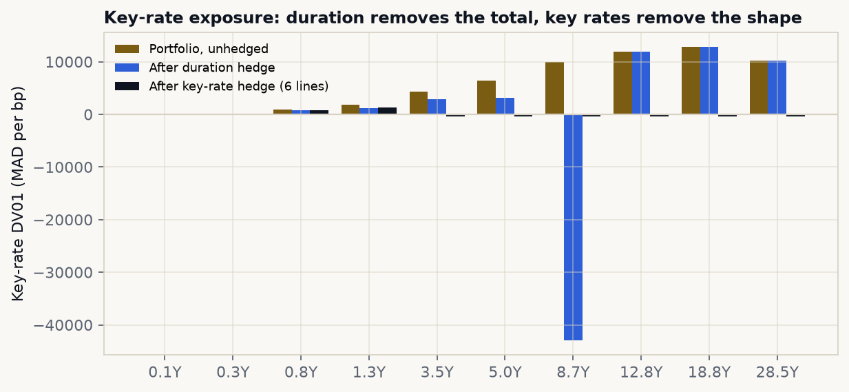
Duration zeroes the total by concentrating the exposure at 8.7Y; the key-rate hedge removes the shape. The 8.7Y bar is -42.9k MAD/bp after the duration hedge.
The unhedged book has positive exposure at every tenor, rising to +12.8k at 18.8Y. After the duration hedge, the total is zero — but the 8.7Y point flips to -42.9k MAD/bp while the long end is untouched. The hedge did not remove rate risk; it concentrated it at one point on the curve, in the opposite direction. A 1 bp move at 8.7Y now costs more than a 1 bp move anywhere else gains.
Two other residuals matter:
- Convexity. The DV01-matched short leaves +3.40B of dollar convexity, 41% of the 8.21B book. The portfolio is more convex per unit of DV01 than the 8.7Y bullet, because it is a ladder across 0.8 to 28.5 years. At ±100 bp the hedged book gains +190k / +152k MAD — positive in both directions. That is a long-volatility position nobody asked for.
- Curve shape. The single-instrument hedge has no opinion about slope; it simply shorts the 8.7Y point. A +100 bp steepener (short rates -100 bp, long rates +100 bp) costs the hedged book -2.18M MAD, while the unhedged book gains +501k. A +100 bp belly move at 12.76Y adds +630k MAD. The hedge can be worse than no hedge under the right curve move.
The execution problem is just as serious. A 76.9M short in one line is 94% of the book’s market value and 7.7 times the book’s 10M per-line holding. Under a 10M per-line cap only 13% of this hedge can be placed, leaving 87% of the DV01 unhedged.
The duration-plus-convexity hedge
To neutralize both DV01 and convexity, I used two instruments — the 5.01-year 3.09% line and the 18.84-year 4.09% line — and solved the 2×2 system:
Short 25.2M MAD of the 5.01Y line; short 34.9M MAD of the 18.84Y line.
Residual DV01 is 1 MAD/bp and residual dollar convexity is zero (to numerical precision). The stress table is the honest scorecard. I use a 12.76-year belly, not a 15-year hump, because 12.76Y is an observed key tenor and 15Y is not.
| Scenario | Unhedged | Duration | Duration + convexity | Key-rate 6 |
|---|---|---|---|---|
| Parallel -100 bp | +6,277k | +190k | +4k | -13k |
| Parallel +100 bp | -5,453k | +152k | -3k | -11k |
| Steepener +100 bp | +501k | -2,177k | +95k | +160k |
| Flattener -100 bp | -215k | +2,369k | +113k | -169k |
| Belly +100 bp (12.76Y) | -3,036k | +630k | +369k | +86k |
At ±100 bp parallel, the duration-plus-convexity book moves by -2.9k / +3.8k MAD — effectively flat. The duration-only book still gains in both directions, which is the convexity bet showing through. But a +100 bp belly at 12.76Y moves the two-instrument book by +369k MAD. The duration-only book is at +630k, and even the unhedged book loses 3.04M to that move. This is the trade: a parallel-neutral book is not a curve-neutral book. The two-instrument hedge buys parallel and convexity neutrality and sells shape neutrality.
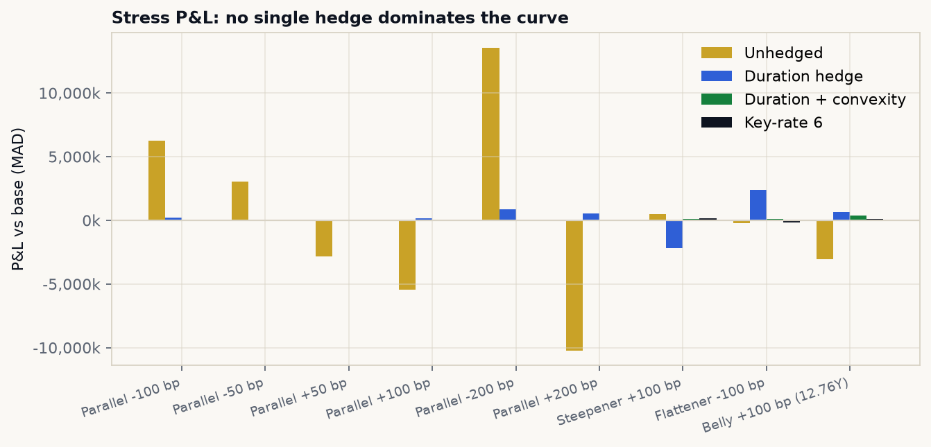
The unhedged book dominates the scale. The point is the residual shape risk in the other bars: duration removes the level, duration-plus-convexity removes the parallel curvature, and both leave the belly.
The key-rate hedge
The earlier version of this note said the next step was a key-rate hedge with three or more instruments, then stopped. This section builds it. With N instruments you can zero N key-rate exposures. The book has eight non-trivial knots (0.83Y to 28.53Y), so a three-instrument hedge is necessarily partial; the useful question is how much it leaves, not whether it is “the” hedge.
I solve a duration-neutral least-squares key-rate hedge: choose signed notionals that minimize the squared residual key-rate DV01 across all tenors, subject to the residual total DV01 being zero. The three-line version uses 12.76Y, 18.84Y and 28.53Y. The six-line version adds 3.50Y, 5.01Y and 8.68Y.
| Hedge | Lines | Gross short | Residual DV01 | Residual convexity | Belly +100 | Steepener +100 |
|---|---|---|---|---|---|---|
| Duration | 8.68Y | 76.9M | 0 | +3.40B | +630k | -2,177k |
| Duration + convexity | 5.01Y, 18.84Y | 60.1M | 1 | 0 | +369k | +95k |
| Key-rate 3 | 12.76Y, 18.84Y, 28.53Y | 43.2M | 0 | -2.19B | +230k | +1,418k |
| Key-rate 6 | 3.50Y–28.53Y | 63.0M | 0 | -0.25B | +86k | +160k |
The three-line hedge is a real improvement on duration-only — it cuts gross short from 76.9M to 43.2M and belly P&L from +630k to +230k — but it leaves a negative convexity residual of -2.19B and a steepener exposure of +1.42M. It is not a finished hedge. The six-line hedge shorts roughly 10M in each of the six liquid lines. It zeroes DV01, cuts residual convexity to -0.25B, and reduces the belly move to +86k. Its residual key-rate exposure is the two short bills (0.83Y and 1.33Y), which are deliberately outside the hedge set: adding them would replicate the book, not hedge it.
The six-line hedge is also the most executable. At a 10M per-line cap it places 95% of its intended gross short and leaves 3.7% of DV01; the duration short places 13% and leaves 87%. That is the practical argument for key rates: the hedge that looks best on a single DV01 number is the one that cannot be put on.
Size, liquidity and financing
BAM’s reference table reports transaction volume as 0.00 for every line. It is a reference curve, not a depth measure, so I cannot prove that 77M is executable. I can show how each hedge degrades under a per-line cap. The caps below are illustrative, not observed: 10M is the book’s own per-line holding, 20M is twice that, and 40M is four times.
| Hedge | Gross short | Lines | Gross / book | Cap 10M executed | Residual DV01 at cap | Financing / month (50 bp) |
|---|---|---|---|---|---|---|
| Duration | 76.9M | 1 | 1.95× | 13% | 50.8k (87%) | 32k |
| Duration + convexity | 60.1M | 2 | 1.74× | 33% | 40.3k (69%) | 25k |
| Key-rate 3 | 43.2M | 3 | 1.53× | 69% | 17.8k (31%) | 18k |
| Key-rate 6 | 63.0M | 6 | 1.77× | 95% | 2.2k (3.7%) | 26k |
Financing is the other constraint. At a 50 bp net spread (the short rebate earns the policy rate, the repo spread is 50 bp), the six-line hedge costs about 26k MAD per month, or 0.45 bp of book DV01. At a 2.75% all-in repo rate (the 2.25% policy rate plus 50 bp), the same hedge costs about 144k MAD per month, or 2.47 bp of DV01. The duration short costs 32k / 176k per month at the same two assumptions. A hedge that saves less than 2-3 bp per month is not worth the financing; that is a real hurdle, not a rounding error.
Leverage is similar across the hedges — gross short is 1.5-1.9 times the book — but concentration is not. The duration hedge puts 7.7 line-equivalents into one line; the six-line key-rate hedge puts about one line-equivalent into each of six lines. If the book itself is executable, the key-rate hedge is the one that is executable at size.
Out-of-sample: does the hedge survive a moving curve?
A one-day hedge is a snapshot. To test the hedges as the curve moved, I downloaded 132 weekday BAM fixings from 1 April to 16 October 2026. Of these, 107 carry the full ten-point cross-section; I use those 107 fixings (106 daily intervals) and drop the sparse dates rather than fit a six-to-nine point curve whose decay constants are not identified. The book is a constant-maturity eight-line book; coupons are set from the first day’s fitted curve, so no future information enters the position. At each rebalance the hedge is re-solved on that day’s curve and held until the next rebalance. P&L is a full reprice, not a duration approximation, and includes coupon cash flows; without the coupon cash, the mechanical price drop at an ex-date would contaminate the hedge P&L. I charge 2 bp one-way on hedge turnover and a 50 bp annual net financing spread on the short notional.
The key-rate grid is fixed at the 16 October tenors for the whole backtest. The published set of reference maturities changes through time; re-basing the triangular bumps on each day’s sparse set makes the hedge matrix ill-conditioned (on days with only six reference points it produced absurd notionals). That is a data caveat as well as a modelling choice.
| Book | Daily P&L std | Annualized vol | Worst day | 95% VaR | Cumulative |
|---|---|---|---|---|---|
| Unhedged | 112k | 1.77M | -550k | -196k | +51k |
| Duration | 50k | 0.79M | -144k | -93k | -550k |
| Duration + convexity | 8k | 0.13M | -22k | -9k | +330k |
| Key-rate 6 | 6k | 0.09M | -19k | -8k | +191k |
The duration-only hedge cuts daily P&L standard deviation from 112k to 50k, but it still leaves the largest residual among the hedges; the reason is in the stress table, not the average: it is short 8.68Y, so a steepener or a belly move still moves the book. Duration-plus-convexity cuts the volatility to 8k. The six-line key-rate hedge cuts it to 6k, a 95% reduction relative to unhedged and an 89% reduction relative to duration-only; its 95% VaR is -8k versus -196k unhedged. Weekly rebalancing leaves the risk profile essentially unchanged (6k standard deviation, +191k cumulative) and the transaction cost is 13.8k either way, so the operational recommendation is weekly, not daily.
This is not a profitability claim. The unhedged book ended +51k after carry; the duration hedge lost 550k after financing and costs; the duration-plus-convexity and key-rate books ended +330k and +191k. The point is the shape of the residual, not the sign of the cumulative P&L. A hedge that is flat on 16 October but has 50k daily volatility is still not a hedge a risk committee should accept.
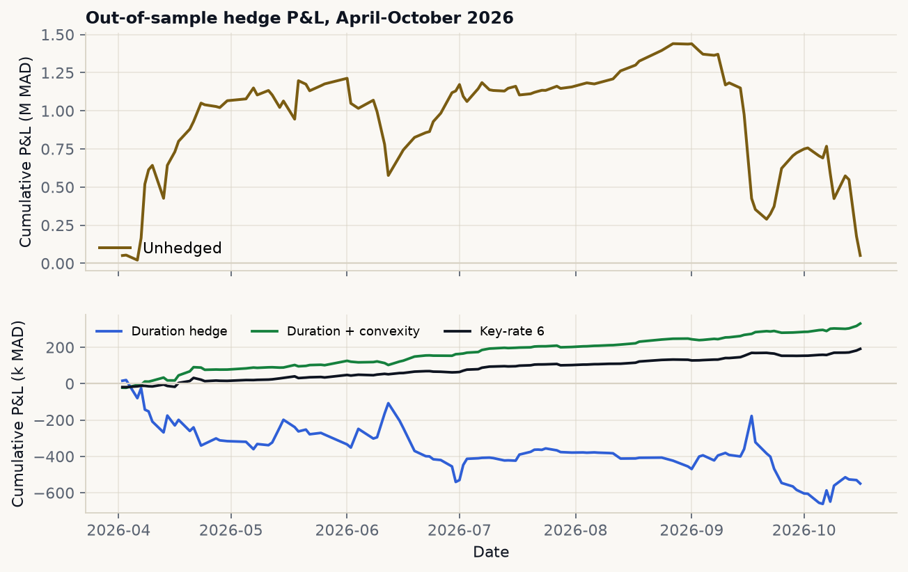
Top: unhedged book. Bottom: the three hedges, net of 2 bp transaction costs and a 50 bp financing spread. The duration short leaves 50k of daily volatility; the key-rate hedge leaves 6k and stays closest to zero.
Move the curve yourself
Scroll to load the curve model.
Drag the three sliders — parallel, slope, belly — and toggle between the unhedged book, the duration hedge, the duration-plus-convexity hedge, and the three- and six-line key-rate hedges. The belly slider now peaks at 12.76Y, one of the observed key tenors. The widget reprices every cash flow against the shifted NSS curve, using the same bond definitions and hedge notionals as the Python engine. The P&L is not a duration approximation; it is a full reprice.
Limitations
- The fit is thin. NSS has six parameters and ten points. The in-sample 3.85 bp is not an out-of-sample number; LOOCV is 30.6 bp. The four-parameter NS robustness check gives the same hedges, but the curve level at the 28.5-year point is genuinely uncertain.
- BAM reference yields are indicative, not executable. They are a secondary-market reference, not a bid or an offer. The table reports zero transaction volume, so depth cannot be inferred from it.
- The backtest is one sample. It covers 6.4 months of 2026, not a full rate cycle. The book is constant-maturity and the coupons are set at the start; no taxes, coupon reinvestment, or intraday execution are modelled. Costs and financing are assumptions, not dealer quotes.
- Short-sale constraints are not modelled. The hedge assumes the lines can be borrowed. In practice, Moroccan sovereign repo and securities lending are thin; a desk may not be able to short the 28.5-year line at all.
- Key-rate DV01 uses triangular bumps between reference tenors. That is a convention, not a unique decomposition; a different bump shape changes the attribution, not the total DV01. The capacity caps are illustrative, not observed market depth.
The point of the project is not that one hedge is “correct.” It is that DV01 is a scalar summary of a curve, and two books with the same DV01 can have completely different risk. Duration gets you to zero. Key rates tell you what you still own. A size cap tells you whether you can own it at all.
Reproducibility
cd mad-curve-lab
python3 bam_curve.py selftest
python3 bam_curve.py analyze
python3 bam_curve.py analyze --model ns --out outputs_ns
python3 bam_curve.py backtest
Data: Bank Al-Maghrib, Taux de référence des bons du Trésor, secondary market, value date 16 October 2026; daily history 1 April - 16 October 2026. Policy rate: Bank Al-Maghrib, 2.25%, accessed October 2026. Source page: bkam.ma → Marchés → Principaux indicateurs → Marché obligataire → Marché des bons du Trésor → Marché secondaire. The raw CSV is committed under data/bam_reference_2026-10-16.csv; the daily history is under data/history/; outputs/ contains the analytics, the stress table, the backtest and the widget payload. The engine, data and outputs live in the companion mad-curve-lab repository.
Not investment advice. This is a risk-management exercise on public reference data, not a recommendation on any security.
